RF Signals and Modulation

Wireless data must travel through free space, without the constraints and protection of a wire. In the free space environment, many variables can affect the data and its delivery. To minimize the variables, wireless engineering efforts must focus on two things:

• Wireless devices must adhere to a common standard.
• Wireless coverage must exist in the area where devices are expected.

---

The sender (a transmitter) can send an alternating current into a section of wire (an antenna), which sets up moving electric and magnetic fields that propagate out and away as traveling waves. The electric and magnetic fields travel along together and are always at right ingles to each other.

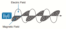
The signal must keep changing, or alternating, by cycling up and down, to keep the electric and magnetic fields cycling and pushing ever outward. Electromagnetic waves travel by expanding in all directions away from the antenna, in all three dimensions.

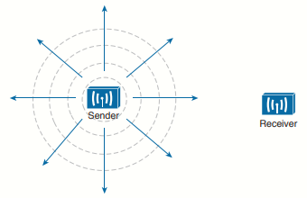
The idealistic antenna does not exist, but serves as a reference point to understand wave propagation.

As the electromagnetic waves reach the receiver's antenna, they induce an electrical signal. If everything works right, the received signal will be a reasonable copy of the original transmitted signal.

---

Frequency

The frequency of the wave is the number of times the signal makes one complete up and down cycle in 1 second. 

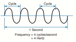
A hertz (Hz) is the most commonly used frequency unit and is nothing other than one cycle per second.

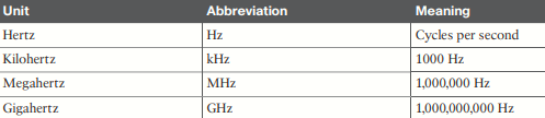
On the continuous frequency spectrum, the frequency range from around 3 kHz to 300 GHz is commonly called radio frequency (RF). The microwave category contains the two main frequency ranges that are used for wireless LAN communication: 2.4 and 5 GHz.

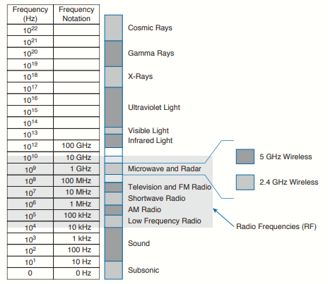
Because a range of frequencies might be used for the same purpose, it is customary to refer to the range as a band of frequencies. One of the two main frequency ranges used for wireless LAN communication lies between 2.400 and 2.4835 GHz. This is usually called the 2.4-GHz band, even though it does not encompass the entire range between 2.4 and 2.5 GHz. It is much more convenient to refer to the band name instead of the specific range of frequencies included.

The other wireless LAN range is usually called the 5-GHz band because it lies between 5.150 and 5.825 GHz. The 5-GHz band actually contains the following four separate and distinct bands (it is interesting that the 5-GHz band can contain several smaller bands; remember that the term band is simply a relative term that is used for convenience):

• 5.150 to 5.250 GHz
• 5.250 to 5.350 GHz
• 5.470 to 5.725 GHz
• 5.725 to 5.825 GHz

A frequency band contains a continuous range of frequencies. If two devices require a single frequency for a wireless link between them, which frequency can they use? Beyond that, how many unique frequencies can be used within a band?

To keep everything orderly and compatible, bands are usually divided up into a number of distinct channels. Each channel is known by a channel number and is assigned to a specific frequency. As long as the channels are defined by a national or international standards
body, they can be used consistently in all locations.

The channel assignment for the 2.4 GHz band that is used for wireless LAN communication contains 14 channels (1 to 14), each asigned a specific frequency. 

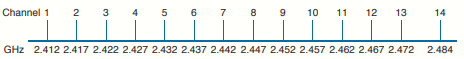
Notice how much easier it is to refer to channel numbers than the frequencies. Also notice how channels are spaced at regular intervals that are 0.005 GHz apart (except for channel 14). The channel spacing is known as the channel separation or channel width.

If devices use a specific frequency for a wireless link, why do the channels need to be spaced apart at all? In practice, an RF signal is not infinitely narrow; instead, it spills above and below a center frequency to some extent, occupying neighboring frequencies, too. It is the center frequency that defines the channel location within the band. The actual frequency range needed for the transmitted signal is known as the signal bandwidth.

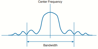
Bandwidth refers to the width of frequency space required within the band. For example, a signal with 22 MHz bandwidth is bounded at 11 MHz above and below the center frequency. In wireless LANs, the signal bandwidth is defined as part of a standard. Even though the signal might extend farther above and below the center frequency than the bandwidth allows, wireless devices will use something called a spectral mask to ignore parts of the signal that fall outside the bandwidth boundaries.

Ideally, the signal bandwidth should be less than the channel width so that a different signal could be transmitted on every possible channel with no chance that two signals could overlap and interfere with each other. The following image shows such a channel spacing, where the signals on adjacent channels do not overlap. A signal can exist on every possible channel without overlapping with others.

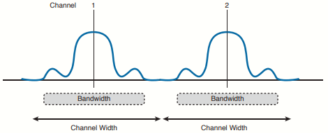
However, you should not assume that signals centered on the standardized channel assignments will not overlap with each other. It is entirely possible that the channels in a band are narrower than the signal bandwidth:

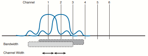
Notice how two signals have been centered on adjacent channels numbers 1 and 2, but they almost entirely overlap each other! The problem is that the signal bandwidth is slightly wider than four channels. In this case, signals centered on adjacent channels cannot possibly coexist without overlapping and interfering. Instead, the signals must be placed on more distant channels to prevent overlapping, thus limiting the number of channels that can be used in the band.

---

Phase

The phase of a signal is a measure of shift in time relative to the start of a cycle. Phase is normally measured in degrees, where 0 degrees is at the start of a cycle, and one complete cycle equals 360 degrees.  A point that is halfway along the cycle is at the 180-degree mark. Because an oscillating signal is cyclic, you can think of the phase traveling around a circle again and again. When two identical signals are produced at exactly the same time, their cycles match up and they are said to be in phase with each other. If one signal is delayed from the other, the two signals are said to be out of phase:

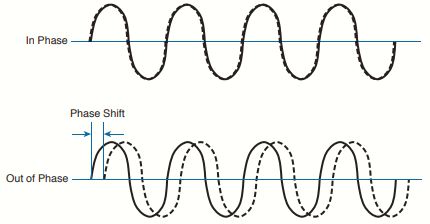
Phase becomes important as RF signals are received. Signals that are in phase tend to add together, whereas signals that are 180 degrees out of phase tend to cancel each other out. 

---

Wavelength

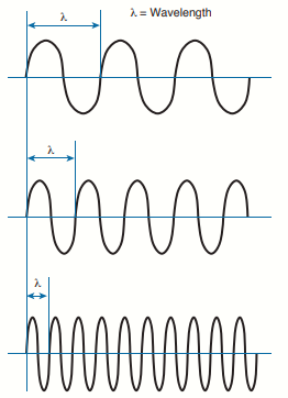
The wavelength is a measure of the physical distance that a wave travels over one complete cycle. Wavelength is usually designated by the Greek symbol lambda (λ). To get a feel for the dimensions of a wireless LAN signal, assuming you could see it as it travels in front of you, a 2.4-GHz signal would have a wavelength of 12,50 cm, while a 5-GHz signal would be 6 inches.

Regardless of the frequency, RF waves travel at a constant speed. In a vacuum, radio waves travel at exactly the speed of light; in air, the
velocity is slightly less than the speed of light. Notice that the wavelength decreases as the frequency increases. As the wave cycles get smaller, they cover less distance. Wavelength becomes useful in the design and placement of antennas.

• Lower frequency (longer wavelength) → travels farther, penetrates walls better (2.4 GHz).

• Higher frequency (shorter wavelength) → attenuates faster, more easily blocked, but allows for smaller antennas and higher data rates (5 GHz, 6 GHz Wi-Fi 6E).

• Antenna size is often proportional to the wavelength

The speed at which RF waves travel (essentially the speed of light) does not influence the data rate in Mbps. What determines Mbps is how much information can be encoded into the signal, which depends on channel bandwidth (e.g., 20, 40, 80, or 160 MHz) and the modulation scheme (how many bits are carried per symbol, such as QPSK, 64-QAM, or 1024-QAM). Higher frequencies like 5 GHz and 6 GHz make it easier to allocate wider channels and use more advanced modulation, so they can achieve much higher Mbps rates than 2.4 GHz, even though the propagation speed of the waves is essentially the same.

---

Understanding RF Power and dB

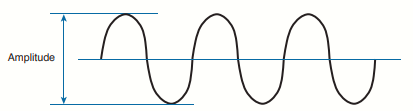
For an RF signal to be transmitted, propagated through free space, received, and understood with any certainty, it must be sent with enough strength or energy to make the journey. This strength can be measured as the amplitude, or the height from the top peak to the bottom peak of the signal’s waveform.

The strength of an RF signal is usually measured by its power, in watts (W). A wireless LAN transmitter usually has a signal strength between 0.1 W (100 mW) and 0.001 W (1 mW).

When power is measured in watts or milliwatts, it is considered to be an absolute power measurement. In other words, something has to measure exactly how much energy is present in the RF signal. This is fairly straightforward when the measurement is taken at the output of a transmitter because the transmit power level is usually known ahead of time.

Sometimes you might need to compare the power level between two different transmitters. For example, suppose that device T1 is transmitting at 1 mW, while T2 is transmitting at 10 mW:

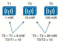
Simple subtraction tells you that T2 is 9 mW stronger than T1. You might also notice that T2 is 10 times stronger than T1.

Now compare transmitters T2 and T3, which use 10 mW and 100 mW, respectively:

Using subtraction, T2 and T3 differ by 90 mW, but T3 is again 10 times stronger than T2. In each instance, subtraction yields a different result than division.

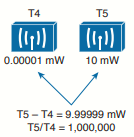
A more surprising example is shown below:

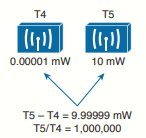
T4 is 0.00001 mW and T5 is 10 mW. Subtracting the two values gives their difference as 9.99999 mW. However, T5 is 1,000,000 times stronger than T4!

Because absolute power values can fall anywhere within a huge range, from a tiny decimal number to hundreds, thousands, or greater values, we need a way to transform the exponential range into a linear one. The logarithm function can be leveraged to do just that. In a nutshell, a logarithm takes values that are orders of magnitude apart (0.001, 0.01, 0.1, 1, 10, 100, and 1000, for example) and spaces them evenly within a reasonable range.

The base-10 logarithm function, denoted by log₁₀, computes how many times 10 can be multiplied by itself to equal a number. For example, log₁₀(10) equals 1 because 10 is used only once to get the result of 10. The log₁₀(100) equals 2 because 10 is multiplied twice (10 × 10), to reach the result of 100. Computing other log₁₀ values is difficult, requiring the use of a calculator.

The decibel (dB) is a handy function that uses logarithms to compare one absolute measurement to another. After each power value has been converted to the same logarithmic scale, the following equation is used to calculate a dB value, where P1 and P2 are the absolute power levels of two sources:

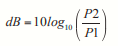
P2 represents the source of interest, and P1 is usually called the reference value or the source of comparison.

Here, the ratio of the two absolute power values is computed first; then the result is converted onto a logarithmic scale.

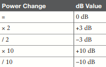
Important dB Laws to Remember

There are three cases where you can use mental math to make power-level comparisons using dB. By adding or subtracting fixed dB amounts, you can compare two power levels through multiplication or division. You should memorize the following three laws, with are based on dB changes of 0, 3, and 10, respectively, and are known as the Law of Zero, Law of 3s, and Law of 10. All other dB cases require a calculator.

• Law of Zero: A value of 0 dB means that the two absolute power values are equal. If the two power values are equal, the ratio inside the logarithm is 1, and the log₁₀(1) is 0. This law is intuitive; if two power levels are the same, one is 0 dB more than the other.
  
  
• Law of 3s: A value of 3 dB means that the power value of interest is double the reference value; a value of –3 dB means the power value of interest is half the reference. When P2 is twice P1, ratio is always 2. Therefore, 10log₁₀(2) = 3 dB. When ratio is 1/2, 10log₁₀(1/2) = -3 dB
  
  Whenever a power level doubles, it increases by 3 dB. Whenever it is cut in half, it decreases by –3 dB.
  
  
• Law of 10s: A value of 10 dB means that the power value of interest is 10 times the reference value; a value of –10 dB means the power value of interest is 1/10 of the reference. When P2 is 10 times P1, the ratio is always 10. Therefore, 10log₁₀(10) = 10 dB. When P2 is one tenth of P1, then the ratio is 1/10 and 10log₁₀(1/10) = –10 dB

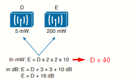
When absolute power values multiply, the dB value is positive and can be added. When the power values divide, the dB value is negative and can be subtracted:

Example:

Comparing Power Against a Reference: dBm

Beyond comparing two transmitting sources, a wireless LAN engineer must be concerned about the RF signal propagating from a transmitter to a receiver. After all, transmitting a signal is meaningless unless someone is there to receive it and make use of it.

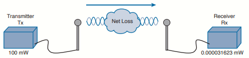
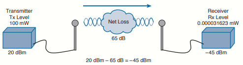
Nothing in the real world is ideal, so assume that something along the path of the signal will induce a net loss. At the receiver, the signal strength will be degraded by some amount. Suppose that you are able to measure the power level leaving the transmitter, which is 100 mW. At the receiver, you measure the power level of the arriving signal. It is an incredibly low 0.000031623 mW.

You could leverage the handy dB formula to compare the received signal strength to the
transmitted signal strength:

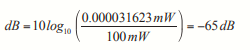
The net loss over the signal path turns out to be a decrease of 65 dB. Knowing that, you decide to try a different transmit power level to see what would happen at the receiver. The best approach is to convert every power level to a dB value and simply add them up along the path.

In wireless networks, power is often expressed in dBm, which is just a logarithmic way of comparing a power level to a fixed reference of 1 milliwatt (mW) (the choice of 1 milliwatt as the reference is really just a convention in RF engineering). The formula is:

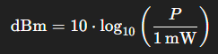
This means you take the power you’re interested in (P), divide it by 1 mW (the reference), and then apply the log scale. For example, if P=100 mW the result is 20 dBm.

Returning to the scenario, notice that the dBm values can be added along the path: The transmitter dBm plus the net loss in dB equals the received signal in dBm.

Measuring Power Changes Along the Signal Path

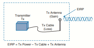
A transmitter, its cable, and its antenna are separate components that together determine the final RF power. While the transmitter produces the signal, the antenna provides gain that increases the signal strength, though it does not generate power itself. Antenna gain is expressed in dB by comparing it to a reference antenna, typically the ideal isotropic antenna, which radiates equally in all directions and serves as a universal benchmark (dBi). The connecting cable introduces some signal loss, specified in dB per unit length. By combining transmitter power, cable loss, and antenna gain, the actual output power radiated—called the effective isotropic radiated power (EIRP)—can be calculated in dBm.

EIRP is a very important parameter because it is regulated by governmental agencies in most countries. In those cases, a system cannot radiate signals higher than a maximum allowable EIRP. To find the EIRP of a system, simply add the transmitter power level to the antenna gain and subtract the cable loss:

EIRP combines values in dBm, dBi, and dB, which can be added or substracted directly when calculating. The only exception is when antenna gain is given in dBd (referenced to a dipole instead of an isotropic antenna). Since a dipole has a gain of 2.14 dBi, you can convert dBd to dBi by simply adding 2.14.

Power-level considerations do not have to stop with the EIRP. You should also be concerned with the complete path of a signal, to make sure that the transmitted signal has sufficient power so that it can effectively reach and be understood by a receiver. This is known
as the link budget. The dB values of gains and losses can be combined over any number of stages along a signal’s path:

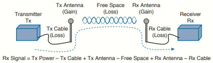
Example (the loss between the two antennas is usually not given, but calculated based on the other values given or as a function of distance and frequency).

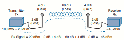
If you always begin with the transmitter power expressed in dBm, it is a simple matter to add or subtract the dB components along the signal path to find the signal strength that arrives at the receiver.

Understanding Power Levels at the Receiver

At the receiving end of the signal path, a receiver expects to find a signal on a predetermined frequency, with enough power to contain useful data. Receivers measure a signal’s power in dBm according to the received signal strength indicator (RSSI) scale.

When you work with wireless LAN devices, the EIRP levels leaving the transmitter’s antenna normally range from 100 mW down to 1 mW. This corresponds to the range +20 dBm down to 0 dBm. At the receiver, the power levels are much, much less, ranging from 1 mW
all the way down to tiny fractions of a milliwatt, approaching 0 mW. The corresponding range of received signal levels is from 0 dBm down to about –100 dBm.

Therefore, the RSSI of a received signal can range from 0 to –100, where 0 is the strongest and –100 is the weakest. The range of RSSI values can vary between one hardware manufacturer and another. RSSI values are supposed to represent dBm values, but the results are not standardized across all receiver manufacturers. An RSSI value can vary from one receiver hardware to another.

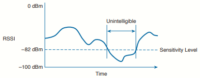
Assuming a transmitter is sending an RF signal with enough power to reach a receiver, what RSSI value is good enough? Every receiver has a sensitivity level or a threshold that divides intelligible, useful signals from unintelligible ones. As long as a signal is received with a power level that is greater than the sensitivity level, chances are that the data from the signal can be understood correctly.

The RSSI value focuses on the expected signal alone, without regard to any other signals that may be received. All other signals that are received on the same frequency as the one you are trying to receive are simply viewed as noise. The noise level, or the average signal strength of the noise, is called the noise floor.

Signal strength must be greater than the noise floor by a decent amount so that it can be received and understood correctly. The difference between the signal and the noise is called the signal-to-noise ratio (SNR), measured in dB. A higher SNR value is preferred.

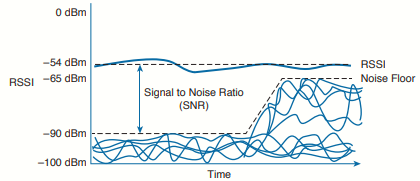
The image above shows the RSSI of a signal compared with the noise floor that is received. The RSSI averages around –54 dBm. On the left side of the graph, the noise floor is –90 dBm. The resulting SNR is –54 dBm – (–90) dBm or 36 dB. Toward the right side of the graph,
the noise floor gradually increases to –65 dBm, reducing the SNR to 11 dB. The signal is so close to the noise that it might not be usable.

---

Carrying Data Over an RF Signal

Up to this point in the chapter, only the RF characteristics of wireless signals have been discussed. The RF signals presented have existed only as simple oscillations in the form of a sine wave. The frequency, amplitude, and phase have all been constant. The steady, predictable frequency is important because a receiver needs to tune to a known frequency to find the signal in the first place.

This basic RF signal is called a carrier signal because it is used to carry other useful information. With AM and FM radio signals, the carrier signal also transports audio signals. TV carrier signals have to carry both audio and video. Wireless LAN carrier signals must carry data.

To add data onto the RF signal, the frequency of the original carrier signal must be preserved. Therefore, there must be some scheme of altering some characteristic of the carrier signal to distinguish a 0 bit from a 1 bit. Whatever scheme is used by the transmitter must
also be used by the receiver so that the data bits can be correctly interpreted.

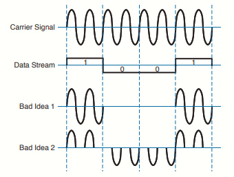
The image above shows a carrier signal with a constant frequency. The data bits 1001 are to be sent over the carrier signal, but how? One idea might be to simply use the value of each data bit to turn the carrier signal off or on. The Bad Idea 1 plot shows the resulting RF signal. A receiver might be able to notice when the signal is present and has an amplitude and correctly interpret 1 bits, but there is no signal to receive during 0 bits. If the signal becomes weak or is not available for some reason, the receiver will incorrectly think that a long string of 0 bits has been transmitted. A different twist might be to transmit only the upper half of the carrier signal during a 1 bit and the lower half during a 0 bit, as shown in the Bad Idea 2 plot. This time, a portion of the signal is always available for the receiver, but the signal becomes impractical to receive because important pieces of each cycle are missing. In addition, it is very difficult to transmit RF with disjointed alternating cycles.

Such naive approaches might not be successful, but they do have the right idea: to alter the carrier signal in a way that indicates the information to be carried. This is known as modulation, where the carrier signal is modulated or changed according to some other source. At the receiver, the process is reversed; demodulation interprets the added information based on changes in the carrier signal.

RF modulation schemes generally have the following goals:

• Carry data at a predefined rate.
• Be reasonably immune to interference and noise.
• Be practical to transmit and receive.

Due to the physical properties of an RF signal, a modulation scheme can alter only the following attributes:

• Frequency (but only varying slightly above or below the carrier frequency).
• Phase
• Amplitude

The modulation techniques require some amount of bandwidth centered on the carrier frequency. This additional bandwidth is partly due to the rate of the data being carried and partly due to the overhead from encoding the data and manipulating the carrier signal. If the data has a relatively low bit rate, such as an audio signal carried over AM or FM radio, the modulation can be straightforward and requires little extra bandwidth. Such signals are called narrowband transmissions.

In contrast, wireless LANs must carry data at high bit rates, requiring more bandwidth for modulation. The end result is that the data being sent is spread out across a range of frequencies. This is known as spread spectrum. At the physical layer, wireless LANs can bebroken down into the following three spread-spectrum categories, which are discussed in subsequent sections:

• Frequency-hopping spread spectrum (FHSS)
• Direct-sequence spread spectrum (DSSS)
• Orthogonal frequency-division multiplexing (OFDM)

FHSS

Early wireless LAN technology took a novel approach as a compromise between avoiding RF interference and needing complex modulation. The wireless band was divided into 79 channels or fewer, with each channel being 1 MHz wide. To avoid narrowband interference, where an interfering signal would affect only a few channels at a time, transmissions would need to continuously “hop” between frequencies all across the band. This is known as frequency-hopping spread spectrum.

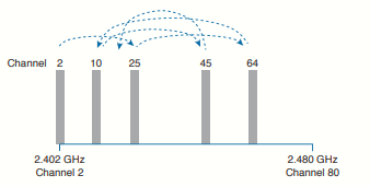
In the image above, the sequence begins on channel 2, then moves to channels 25, 64, 10, 45, and so on, through an entire
predetermined sequence before repeating again. Hopping between channels has to occur at regular intervals so that the transmitter and receiver can stay synchronized. In addition, the hopping order must be worked out in advance so that the receiver can always tune to the correct frequency in use at any given time.

Whatever advantage FHSS gained avoiding interference was lost because of the following limitations:

• Narrow 1-MHz channel bandwidth, limiting the data rate to 1 or 2 Mbps.
• Multiple transmitters in an area could eventually collide and interfere with each other on
  the same channels.

FHSS is rarely used now.

DSSS

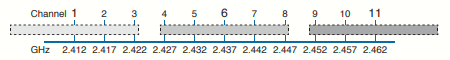
Direct-sequence spread spectrum uses a small number of fixed, wide channels that can support complex modulation schemes and somewhat scalable data rates. The maximum supported data rate is 11 Mbps. Each channel is 22 MHz wide, enough to augment the data by spreading it out and making it more resilient to disruption.

DSSS is used in the 2.4 GHz band. There are 14 possible channels, but only 3 of them that do not overlap (1, 6 and 11):

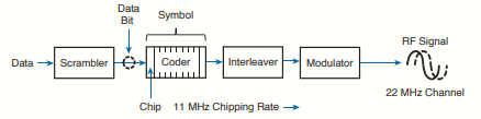
DSSS transmits data in a serial stream, where each data bit is prepared for transmission one at a time. It might seem like a simple matter to transmit the data bits in the order that they are stored or presented to the wireless transmitter; however, RF signals are often affected
by external factors like noise or interference that can garble the data at the receiver. For that reason, a wireless transmitter performs several functions to make the data stream less susceptible to being degraded along the transmission path:

• Scrambler: The data waiting to be sent is first scrambled in a predetermined manner so that it becomes a randomized string of 0 and 1 bits rather than long sequences of 0 or 1 bits.
• Coder: Each data bit is converted into multiple bits of information that contain carefully crafted patterns that can be used to protect against errors due to noise or interference. Each of the new coded bits is called a chip. The complete group of chips representing a data bit is called a symbol. DSSS uses two encoding techniques: Barker codes and Complementary Code Keying (CCK).
• Interleaver: The coded data stream of symbols is spread out into separate blocks so that bursts of interference might affect one block, but not many.
• Modulator: The bits contained in each symbol are used to alter or modulate the phase of the carrier signal. This enables the RF signal to carry the binary data bit values.

At the receiver, the entire process is reversed.

DSSS has evolved over time to increase the data rate that is modulated onto the RF signal. Regardless of the data rate, DSSS always uses a chipping rate of 11 million chips per second.

1-Mbps Data Rate

To minimize the effect of a low SNR and data loss in cases of narrowband interference, each bit of data is encoded as a sequence of 11 bits called a Barker 11 code. The goal is to add enough additional information to each bit of data that its integrity will be preserved when it is sent in a noisy environment.

There are only 2 possible values for the Barker chips, one corresponding to a 0 data bit (10110111000) and one for a 1 data bit (01001000111). The receiver must also expect the Barker chips and convert them back into single bits of data. The number and sequence of the Barker chip bits have been defined to allow data bits to be recovered if some of the chip bits are lost. In fact, up to 9 of the 11 bits in a single chip can be lost before the original data bit cannot be restored.

Each bit in a Barker chip can be transmitted by using the differential binary phase shift keying (DBPSK) modulation scheme. The phase of the carrier signal is shifted or rotated according to the data bit being transmitted, as follows:

• 0: The phase is not changed
• 1: The phase is "rotated" or shifted 180 degrees, such that the original signal is suddenly inverted.

DBPSK can modulate 1 bit of data at a time onto the RF signal. 

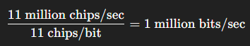
• Chips are sent at 11 million per second (11 Mcps).

• Since each data bit = 11 chips, that’s 1 Mbps:

2-Mbps Data Rate

It is possible to couple the 1-Mbps strategy with a different modulation scheme to double the data rate. As before, each data bit is coded into an 11-bit Barker code with an 11-MHz chipping rate. This time, chips are taken two at a time and modulated onto the carrier signal by using differential quadrature phase shift keying (DQPSK).

The two chips are used to
affect the carrier signal’s phase in four possible ways, each one 90 degrees apart (hence, the
name quadrature). The bit patterns produce the following phase shifts:

• 0° shift → encodes 00

• 90° shift → encodes 01

• 180° shift → encodes 10

• 270° shift → encodes 11

Because DQPSK can modulate data bits in pairs, it is able to transmit twice the data rate of DBPSK, or 2 Mbps.

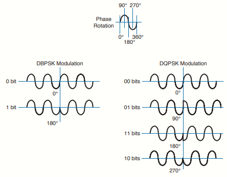
Phase rotations can occur at several points along a cycle; for simplicity, only rotations at the beginning of the cycle (0 degrees) are shown. Notice how abrupt the phase can change, according to the bits being modulated. The receiver must detect these phase changes when it demodulates the signal so that the original data bits can be recovered.

You will often see terms like DBPSK and BPSK mentioned. The two forms reference the same type of modulation (BPSK, in this case), but differ in the reference signal that the receiver uses to detect the phase changes. The nondifferential form (without the initial D) means the receiver must compare with the original premodulated signal to find phase changes. The differential form (with the D) means the receiver must figure out phase changes by comparing with previous phases already seen in the received signal.

5.5-Mbps and 11-Mbps Data Rate

With Barker-11 and a chipping rate of 11 Mcps, you can’t go faster than 2 Mbps, because Barker only allows 1 symbol = 11 chips, and each symbol maxes out at 2 bits (with DQPSK). To go beyond 2 Mbps, they had to change the spreading method.

CCK (Complementary Code Keying) replaces Barker-11 in 802.11b. Instead of spreading each symbol with 11 chips, CCK uses 8-chip codes. The magic: those 8 chips can represent more than just 1 or 2 bits. By carefully choosing the phases in those 8 chips, CCK can encode 4 or 8 bits per symbol while still providing some robustness against noise.

• 5.5 Mbps mode:

  • Each CCK codeword (8 chips) encodes 4 bits.

  • With an 11 Mcps chipping rate:
    
    

    

    
    

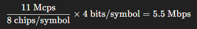
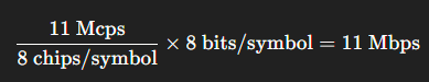
• 11 Mbps mode:

  • Each CCK codeword (8 chips) encodes 8 bits.

  • Same math:
    
    

    

 

In short, they squeezed more speed by packing more data into each spread symbol.

• First, by changing modulation (DBPSK → DQPSK).

• Then, by changing the spreading code (Barker → CCK), which allowed multiple bits per chip sequence instead of just 1 or 2.

OFDM

DSSS spreads the chips of a single data stream into one wide, 22-MHz channel. It is inherently limited to an 11-Mbps data rate because of the consistent 11-MHz chipping rate that feeds into the RF modulation. To scale beyond that limit, a vastly different approach is needed.

Orthogonal frequency-division multiplexing (OFDM) sends data bits in parallel over multiple frequencies, all contained in a single 20-MHz channel. Each channel is divided into 64 subcarriers (also called subchannels or tones) that are spaced 312.5 kHz apart. The
subcarriers are broken down into the following types:

• Guard: 12 subcarriers are used to help set one channel apart from another and to help receivers lock onto the channel.
• Pilot: 4 subcarriers are equally spaced and always transmitted to help receivers evaluate the noise state of the channel.
• Data. 48 subcarriers are devoted to carrying data.

Sometimes you might see OFDM described as having 52 subcarriers (48 for data and 4 for pilot). This is because the 12 guard frequencies are not actually transmitted, but stay silent as channel spacing.

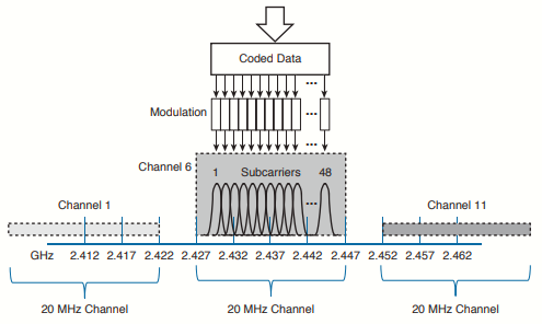
The image shows an example of OFDM where channel 6 in the 2.4 GHz band is 20 MHz wide with 48 data subcarriers. OFDM is named for the way it takes one channel and divides it into a set of distinct frequencies for its subcarriers. Notice that the subcarriers appear to
be spaced too close together, causing them to overlap. In fact, that is the case, but instead of interfering with each other, the overlapped portions are aligned so that they cancel most of the potential interference.

OFDM has the usual scrambling, coding, interleaving, and modulating functions, but it gains its scalability by leveraging so many data subcarriers in parallel. Even though the data rates through each subcarrier are relatively low, the sum of all subcarriers results in a high aggregate data rate.

OFDM offers many different data rates through several different modulation schemes. Because OFDM is concerned with moving data in parallel at higher rates, the amount of information that is repeated for resilience can be varied. The coders used with OFDM are named according to the fraction of symbols that are new or unique, and not repeated. For example, BPSK 1/2 designates that one half of the bits are new and one half are repeated. BPSK 3/4 uses a coder that presents three-fourths new data and repeats only one fourth. As a rule of thumb, a greater fraction means a greater data rate, but a lower tolerance for errors.

At the low end of the range, the familiar BPSK modulation can be used along with two different coder ratios. In this case, OFDM still uses 48 subchannels or tones, with a reduced tone rate of 250 Kbps. OFDM with BPSK 1/2 results in a 6-Mbps data rate, whereas BPSK
3/4 gives 9 Mbps. QPSK 1/2 and 3/4 can be used to increase the data rate to 12 and 18 Mbps, respectively.

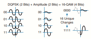
Recall that QPSK uses 2 data bits to modulate the RF signal, resulting in four possible phase shifts. To achieve data rates greater than 18 Mbps, more bits must be used to modulate the signal. Quadrature amplitude modulation (QAM) combines QPSK phase shifting (quadrature) with multiple amplitude levels to get a greater number of unique alterations to the signal. For example, 16-QAM uses 2 bits to select the QPSK phase rotation and 2 bits to select the amplitude level, giving 4 bits or 16 unique modulation changes. 16-QAM:

The number of possible outcomes is always given as a prefix to the QAM name, followed by the coder ratio of new data. In other words, 16-QAM is available in 1/2 and 3/4, providing data rates of 24 and 36 Mbps, respectively. Beyond that, 64-QAM uses 8 phase shifts and 8 amplitude levels to produce 64 unique modulation changes. The 64-QAM 2/3 and 64-QAM 3/4 methods offer 48 and 54 Mbps, respectively.

The same scheme is extended even further with 256-QAM 3/4 and 256-QAM 5/6. As the 256 prefix denotes, 16 different phase shifts and 16 different amplitude levels are combined to produce 256 unique modulation changes, effectively encoding 8 bits of data at a time. With so many shifts and levels in use, receivers can have a difficult job determining the original transmitted values accurately—especially when noise is present. As the modulation schemes get more complex (the QAM prefix gets higher), the signal-to-noise ratio must become greater.

Modulation Summary

• B in DBPSK stands for binary (two outcomes).
• Q in DQPSK stands for quadrature (four outcomes).
• CCK is coupled with QPSK and replaces Barker 11 to go a bit faster.
• OFDM generally wins out, except at the two slowest BPSK methods, which sit between the two CCK methods.
• QAM leverages both phase and amplitude changes to move the greatest amount of data.
• Higher fractions mean higher data rates.

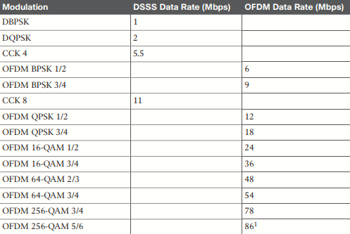
_{¹ The OFDM 256-QAM 5/6 data rate is approximate but is not supported with a single spatial stream.}

To pass data over an RF signal successfully, both a transmitter and receiver have to use the same modulation method. In addition, the pair should use the best data rate possible, given their current environment. If they are located in a noisy environment, where a low SNR or a low RSSI might result, a lower data rate might be preferable. If not, a higher data rate is better.

With so many possible modulation methods available, how do the transmitter and receiver select a common method to use? To complicate things, the transmitter, the receiver, or both might be mobile. As they move around, the SNR and RSSI conditions will likely change from one moment to the next. The most effective approach is to have the transmitter and receiver negotiate a modulation method (and the resulting data rate) dynamically, based on current RF conditions.