
Lab - Implement Multi-Area OSPFv2
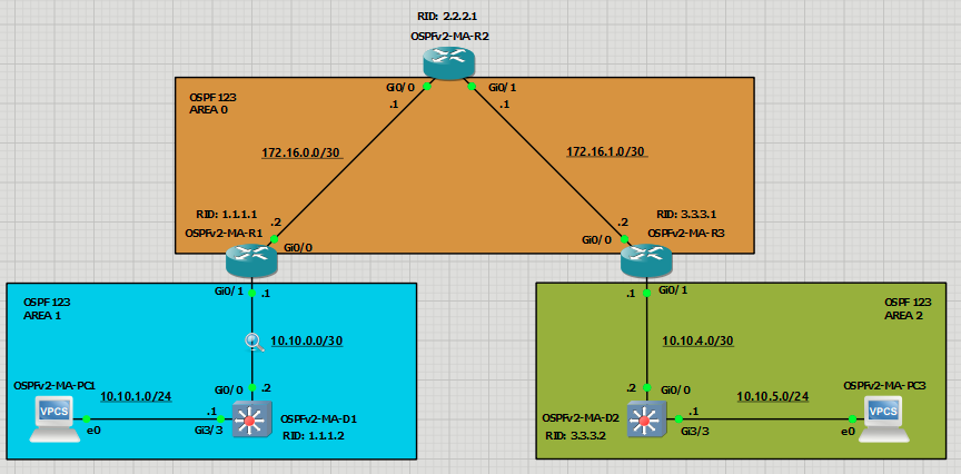
Topology
Addressing Table
| Device | Interface | IPv4 Address |
|---|---|---|
| R1 | G0/0/0 | 172.16.0.2/30 |
| G0/0/1 | 10.10.0.1/30 | |
| R2 | Lo0 | 209.165.200.225/27 |
| G0/0/0 | 172.16.0.1/30 | |
| G0/0/1 | 172.16.1.1/30 | |
| R3 | G0/0/0 | 172.16.1.2/30 |
| G0/0/1 | 10.10.4.1/30 | |
| D1 | G1/0/11 | 10.10.0.2/30 |
| G1/0/23 | 10.10.1.1/24 | |
| D2 | G1/0/11 | 10.10.4.2/30 |
| G1/0/23 | 10.10.5.1/24 | |
| PC1 | NIC | 10.10.1.10/24 |
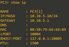
| PC2 | NIC | 10.10.5.10/24 |
Objectives
- Part 1: Build the Network and Configure Basic Device Settings and Interface Addressing
- Part 2: Configure and Verify Multiarea OSPF for IPv4 on R1, D1, and D2
- Part 3: Exploring Link State Announcements
Background / Scenario
To make OSPF more efficient and scalable, OSPF supports hierarchical routing using the areas. An OSPF area is a group of routers that share the same link-state information in their link-state databases (LSDBs). When a large OSPF area is divided into smaller areas, it is called multiarea OSPF. Multi-area OSPF is useful in larger network deployments to reduce processing and memory overhead.
In this lab you will configure multiarea OSPF version 2 for IPv4. This lab was specifically designed to use three routers and two Layer 3 switches.
Note: This lab is an exercise in developing, deploying, and verifying how multiarea OSPF operates and does not reflect networking best practices.
Required Resources - Sergio Jimenez's Version
For this lab I am using GNS3 where I have deployed:
- 3 IOSv 15.9(3)M9 routers
- 2 IOSvL2 15.2 switches
- 2 VPCs
Instructions
Part 1: Configure basic settings for the routers and switches
OSPFv2-MA-R1
hostname R1
no ip domain lookup
line con 0
 logging sync
 exec-time 0 0
 exit
banner motd # This is R1, Implement Multi-Area OSPFv2 Lab #
interface g0/0
 ip add 172.16.0.2 255.255.255.252
 no shut
 exit
interface g0/1
 ip address 10.10.0.1 255.255.255.252
 no shut
OSPFv2-MA-R2
hostname R2
no ip domain lookup
line con 0
logging sync
exec-time 0 0
exit
banner motd # This is R2, Implement Multi-Area OSPFv2 Lab #
interface g0/0
 ip add 172.16.0.1 255.255.255.252
 no shut
 exit
interface g0/1
 ip address 172.16.1.1 255.255.255.252
 no shut
 exit
interface lo0
 ip add 209.165.200.225 255.255.255.224
 exit
OSPFv2-MA-R3
hostname R3
no ip domain lookup
line con 0
 logging sync
 exec-time 0 0
 exit
banner motd # This is R3, Implement Multi-Area OSPFv2 Lab #
interface g0/0
 ip add 172.16.1.2 255.255.255.252
 no shut
 exit
interface g0/1
 ip address 10.10.4.1 255.255.255.252
 no shut
 exit
OSPFv2-MA-D1
hostname D1
no ip domain lookup
line con 0
exec-timeout 0 0
logging synchronous
exit
banner motd # This is D1, Implement Multi-Area OSPFv2 Lab #
interface g0/0
 no switchport
 ip address 10.10.0.2 255.255.255.252
 no shut
 exit
interface g3/3
 no switchport
 ip address 10.10.1.1 255.255.255.0
 no shut
 exit
OSPFv2-MA-D2
hostname D2
no ip domain lookup
line con 0
 logging sync
 exec-time 0 0
 exit
banner motd # This is D2, Implement Multi-Area OSPFv2 Lab #
interface g0/0
 no switchport
 ip address 10.10.4.2 255.255.255.252
 no shut
 exit
interface g3/3
 no switchport
 ip address 10.10.5.1 255.255.255.0
 no shut
 exit
Verify direct connectivity between all five devices. R1 is shown as an example.
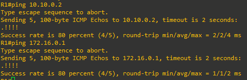
All five devices should be able to reach the other directly connected networks.
Part 2: Configure Multiarea OSPFv2
In this part, you will implement multiarea OSPF. Multiarea OSPF defines a two-layer area hierarchy using a backbone area interconnecting regular areas. This is useful in larger network deployments to reduce processing and memory overhead.
In this topology, OSPF has the following three areas defined:
- Area 0 – The backbone area. All regular areas should connect to the backbone area.
- Area 1 and Area 2 – Regular OSPF areas that connect to the backbone area.
The routers and switches in the topology are used in the following roles:
- Internal routers – R2 is an internal router in Area 0, D1 is internal in Area 1, and D2 is internal in Area 2.
- Backbone routers – R1, R2, and R3 are backbone routers as they all have interfaces in Area 0.
- Area Border routers (ABRs) – R1 and R3 are ABRs because they connect regular areas (i.e., Area 1 and Area 2) to the backbone Area 0.
- Autonomous System Boundary router (ASBR) – R2 is an ASBR because it connects to another non-OSPF network.
Recall that OSPF can be enabled using the traditional network router configuration command or by using the ip ospf process-id area area-id interface configuration command. Although the interface method is simpler, the OSPF routing configuration commands are applied to individual interfaces and not conveniently found in a central location. Therefore, in this lab, we will implement multiarea OSPF using wildcard masks.
You will now configure multiarea OSPF on all five devices starting with D1. You will also configure router IDs, reference bandwidths, and default route propagation.
Note: The verification output displayed in the following part assumes that the devices have been configured in the prescribed order. The output will vary if all devices are configured simultaneously.
Step 1: Implement OSPF on D1 using wildcard masks.
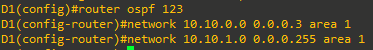
D1 will advertise its OSPF networks using the network router configuration command and wildcard masks. D1 is an internal router in Area 1. Therefore, both network commands will be configured for Area 1.
- Layer 3 switches are not enabled to perform routing by default. Therefore, routing must be enabled using the
ip routingglobal configuration command.
D1(config)# ip routing -
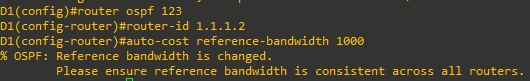
Next, enter the OSPF router configuration mode using process ID 123, assign D1 the router ID 1.1.1.2. You will also set the reference bandwidth to distinguish between Gigabit Ethernet and FastEthernet interfaces. Changing the reference bandwidth to a higher value allows for a differentiation of cost between higher-speed interfaces.

Note: Setting the reference cost value too high may cause issues with low-bandwidth interfaces.
-
Configure D1 to advertise the FastEthernet 0/5 interface 10.10.0.0/30 network in OSPF Area 1. The wildcard mask can be calculated by deducting the subnet mask (i.e., /30 = 255.255.255.252) from 255.255.255.255, resulting in a wildcard mask of 0.0.0.3. Next, configure D1 to advertise its G3/3 interface 10.10.1.0/24 network in OSPF Area 1 and return to privileged EXEC mode.
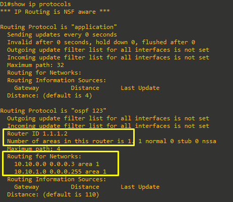
- Verify the OSPF configuration on D1 using the
show ip protocolscommand

The output confirms the router ID, and the number of areas, and the networks advertised. Notice there are no Routing Information Sources because there are no OSPF neighbors.
-
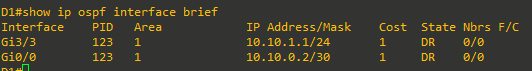
Verify the OSPF interfaces using the
show ip ospf interface briefcommand.
The output confirms that both G3/3 and G0/0 interfaces were correctly assigned to Area 1.
- Finally, verify the OSPF routes in the routing table using the
show ip route ospfcommand.
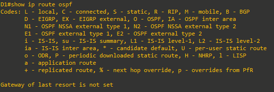
Notice that no routes are displayed. This is because D1 does not yet have an OSPF neighbor.


Step 2: Implement OSPF on R1
Next, configure R1. R1 is an ABR with an interface in Area 1 and the other interface in the backbone.
-
Enter the OSPF router configuration mode using process ID 123, assign R1 the router ID 1.1.1.1, and set the reference bandwidth to distinguish between Gigabit Ethernet and FastEthernet interfaces. Configure R1 to advertise the G0/0 interface 172.16.0.0/30 network in OSPF Area 0. Advertise the G0/1 interface 10.10.0.0/30 network in OSPF Area 1 and return to privileged EXEC mode.
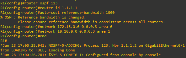
Notice the informational message stating that a neighbor adjacency has been established with D1 (i.e., 1.1.1.2).
- Verify the OSPF configuration on R1 using the
show ip protocolscommand.
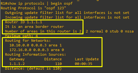
Like the previous output of D1, this output confirms the router ID, and the networks advertised. However, notice that it also explicitly states that R1 is an area border router (ABR), that it is in two areas, and that it has established an adjacency and exchanged routing information with D2 (i.e., 1.1.1.2).
-
Verify that the reference bandwidth has been changed using the
show ip ospf | begin Refcommand.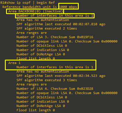
The output confirms that the reference bandwidth has been changed to distinguish GigabitEthernet interfaces. The output also confirms that R1 is in two areas and has two link-state databases (LSDBs).
Note: Area 0 is currently inactive because there are no other peers configured yet.
-
Verify the active OSPF interfaces and assigned areas using the
show ip ospf interface briefcommand.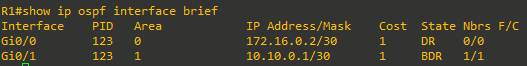
The output confirms the interfaces, areas, and IP addresses. -
Verify which OSPF neighbors R1 has established an adjacency with using the
show ip ospf neighborcommand.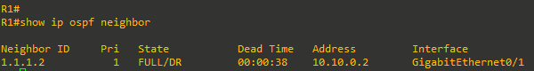
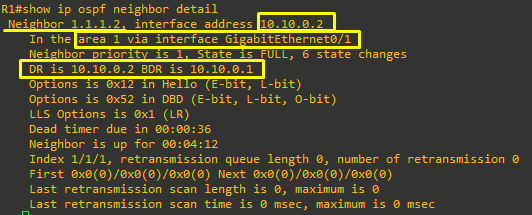
The output confirms that R1 has one neighbor (i.e., 1.1.1.2 = D1), they have a full adjacency established, the IP address of D1 is 10.10.0.2, and R1 can reach D1 using its G0/1 interface.
-
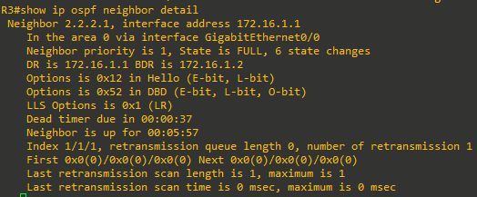
Use the
show ip ospf neighbor detailcommand to get additional information about neighbor adjacencies.
-
Verify the OSPF routes in the routing table using the
show ip route ospfcommand.
The output displays an entry for the D1 LAN. The O designation identifies this as an OSPF internal route. Network routes learned from other OSPF routers in the same area are known as intra-area routes and are identified in the IP routing table with an O.
-
Finally, get detailed information on how R1 learned about the OSPF entry using the
show ip route ospf 10.10.1.0command.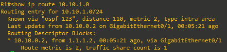
The output confirms that R1 learned about the intra-area route 10.10.1.0 from 10.10.0.2 with a router ID of 1.1.1.2 in OSPF 123.


Step 3: Implement OSPF on R2
Next, configure is R2. R2 is an internal backbone router and will become an ASBR.
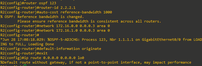
-
Enter the OSPF router configuration mode using process ID 123, assign R2 the router ID 2.2.2.1, and set the reference bandwidth to distinguish between Gigabit Ethernet and FastEthernet interfaces. Configure R2 to advertise its two interfaces in OSPF Area 0 [The output confirms that an adjacency has been established with R1 (i.e., 1.1.1.1)] Note: Alternatively, the two network statements could be combined using network 17.16.0.0 0.0.1.3 area 0. Configure R2 to propagate a default route to the internet. In our lab, the internet is represented as a loopback interface.
- Verify the OSPF configuration on R2 using the
show ip protocolscommand
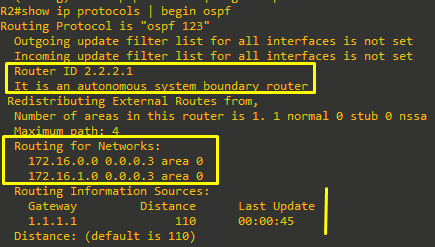
Again, this output confirms the router ID chosen, number of areas R2 is in (i.e., 1), networks advertised, and that it has established an adjacency and exchanged routing information with R1 (i.e., 1.1.1.1). R2 does not have an adjacency with D1 because it is in another area.
Notice as well, that it explicitly states that R2 is an autonomous system boundary router (ASBR). This is because it is now propagating a default route to all other routers in the OSPF domain.
-
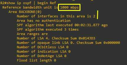
Verify that the reference bandwidth has been changed using the
show ip ospf | begin Refcommand as shown.
The output confirms that the reference bandwidth has been changed and also confirms that R2 has two interfaces in its link-state database (LSDB).
-
Verify the active OSPF interfaces and assigned areas using the
show ip ospf interface briefcommand.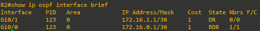
The output confirms that the two interfaces are in Area 0, their IP addresses, state, and neighbors.
-
Verify which OSPF neighbors R2 has established an adjacency using the
show ip ospf neighborcommand.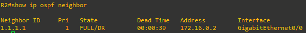
The output confirms that R2 has one neighbor (i.e., 1.1.1.1 = R1) and they have a full adjacency established -
Use the
show ip ospf neighbor detailcommand to get additional information about neighbor adjacencies.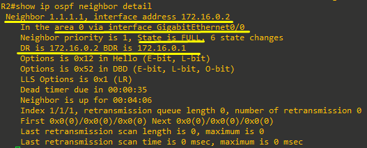
As shown, the output confirms various information about the OSPF neighbor including DR and BDR status.
-
Verify the OSPF routes in the routing table using the
show ip route ospfcommand.
The output displays that there is now a default gateway and two entries for the OSPF Area 1 networks. Notice how these routes are identified as O IA which means they are routes from another area. Network routes learned from OSPF routers in another area using an ABR are known as interarea routes as opposed to intra-area routes.
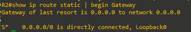
-
Verify the static route entry in the routing table.

-
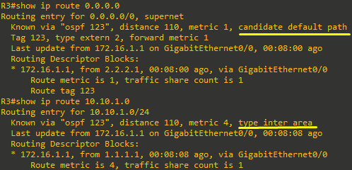
Finally, get detailed information on how R2 learned about the OSPF entry using the
show ip route ospf 10.10.1.0command.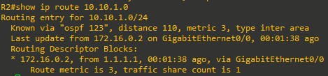
The output confirms that R2 learned about the interarea route 10.10.1.0 from OSPF 123 and specifically from R1, based on the router ID of 1.1.1.1.


Step 4: Implement OSPF on R3
Next to configure is R3. Like R1, R3 is an ABR with an interface in Area 0 and one in Area 2.
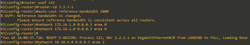
-
Enter the OSPF router configuration mode using process ID 123, assign R3 the router ID 3.3.3.1, and set the reference bandwidth to distinguish between Gigabit Ethernet and FastEthernet interfaces. Ensure reference bandwidth is consistent across all routers. Configure R3 to advertise its interfaces in OSPF Area 0 and Area 2 accordingly and then return to privileged EXEC mode.

-
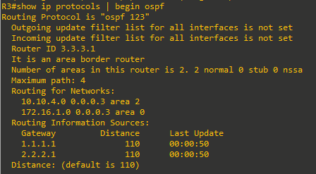
The output confirms the router ID, and that R3 is an ABR, it has interfaces in two areas, the networks it is advertising, and that R3 has R1 (i.e., 1.1.1.1) and R2 (i.e., 2.2.2.1) as sources of routing information.
-
Verify that the reference bandwidth has been changed using the
show ip ospf | begin Refcommand as shown.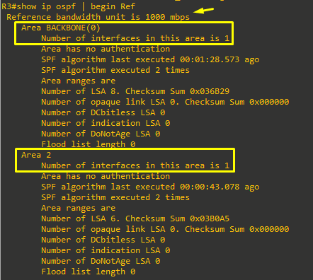
The output confirms that the reference bandwidth has been changed and also confirms that R2 has area information for Area 0 and Area 2.
-
Verify the active OSPF interfaces and assigned areas using the
show ip ospf interface briefcommand.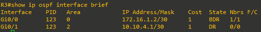
The output confirms the interfaces, process ID, areas, IP addresses, cost, state, and neighbors.
-
Verify which OSPF neighbors R2 has established an adjacency with using the
show ip ospf neighborcommand.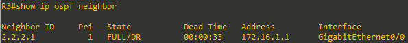
The output confirms that R3 has one neighbor (i.e., 2.2.2.1= R2) and they have a full adjacency established. -
Use the
show ip ospf neighbor detailcommand to get additional information about neighbor adjacencies.

As shown, the output confirms various information about the OSPF neighbor including DR and BDR status.
-
Verify the OSPF routes in the routing table using the
show ip route ospfcommand.
The output verifies that R3 has received a default route from R2, two interarea routes (i.e., O IA routes) and one intra-area OSPF route (i.e., O routes). The O*E2 route indicates that this is an external route that did not originate in OSPF. The asterisk identifies this as a candidate default route.
-
Now get detailed information on how R3 learned about the O E2 and O IA routes.

The output confirms that R3 learned about the default route from R2 (2.2.2.1) and interarea routes from R1 (1.1.1.1) via OSPF.


Step 5: Implement OSPF on D2
Last to configure is D2. Like D1, D2 is an internal router in Area 2.
-
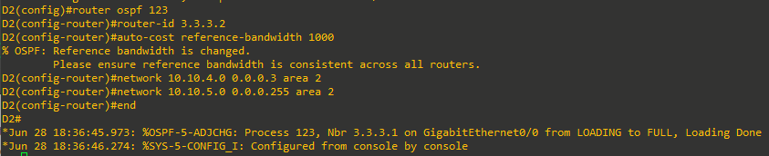
Layer 3 switches are not enabled to perform routing by default. Therefore, routing must be enabled using the
ip routingglobal configuration command. Next, enter the OSPF router configuration mode using process ID 123, assign the D2 the router ID 3.3.3.2, and set the reference bandwidth to distinguish between Gigabit Ethernet and FastEthernet interfaces.Configure D2 to advertise its interfaces in OSPF Area 2 and return to privileged EXEC mode.

- Verify the OSPF configuration on D2 using the
show ip protocolscommand.
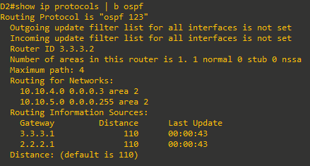
As expected, we can verify the router ID, number of areas, networks being advertised, and routing sources. It may be surprising that R2 (i.e., 2.2.2.1) is displayed as a routing source. The reason is because it is the source of the default route.
-
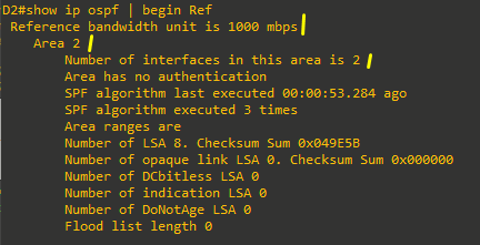
Verify that the reference bandwidth has been changed using the
show ip ospf | begin Refcommand as shown.
-
Verify the active OSPF interfaces and assigned areas using the
show ip ospf interface briefcommand.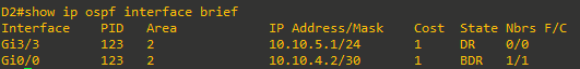
The output confirms that the two interfaces are in Area 2 and their IP addresses are correct.
-
Verify which OSPF neighbors D2 has established an adjacency with using the
show ip ospf neighborcommand.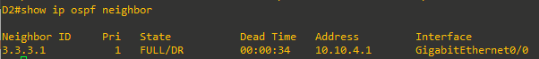
The output confirms that D2 has one neighbor (i.e., 3.3.3.1= R3) and they have a full adjacency established.
-
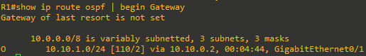
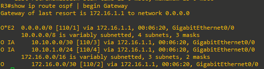
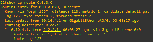
Verify the OSPF routes in the routing table using the
show ip route ospf | begin Gatewaycommand.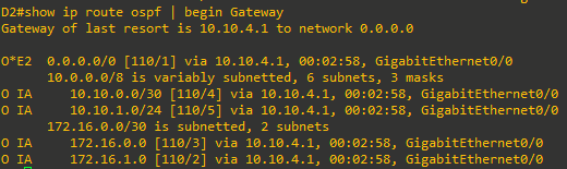
The output displays four interarea routes (i.e., O IA routes) and the OSPF external route from 2.2.2.1(R2).

As we can see, the routing source for the default route is R2 (i.e., 2.2.2.1).


Step 6: Verify end-to-end connectivity
The multiarea OSPF network is now completely configured. We now need to verify the operation of OSPF.
-
From PC1, verify that it has been assigned the correct IP address as listed in the Addressing Table using the
ipconfigWindows command.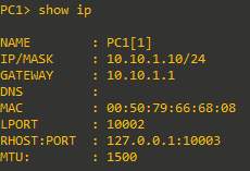

- Verify end-to-end connectivity by pinging PC3.

-
Verify the route taken by doing a traceroute to PC3.
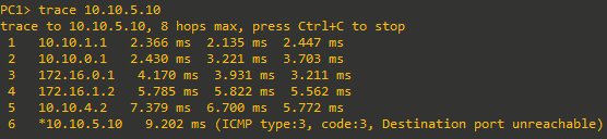

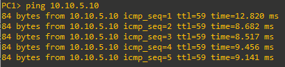

This confirms end-to-end connectivity.
Part 3: Exploring Link State Announcements
In this part, you will verify that the network has converged and explore how link-state advertisements (LSAs) are used as the building blocks for the OSPF link-state database (LSDB).
OSPF routers create LSAs for every directly connected OSPF-enabled interface. It then sends those LSAs to OSPF peers to form adjacencies. Individually, LSAs are database records providing specific OSPF network details. Combined, they describe the entire topology of an OSPF area.
OSPF routers uses six LSA types for IPv4 routing:
• Type 1, router LSA – All OSPF-enabled routers create and send type 1 LSAs. The LSAs are immediately propagated within the area. An ABR does not forward the LSA outside the area.
• Type 2, network LSA – Only a DR generates and advertises a type 2 LSA. The type 2 network LSA lists each of the attached routers that make up the transit network, including the DR itself, and the subnet mask that is used on the link. The DR floods the LSA to all OSPF routers (i.e., 224.0.0.5) on the multiaccess network. The content of the displayed type 2 LSA describes the network segment listing the DR address, the attached routers, and the used subnet mask. This information is used by each router participating in OSPF to build the exact picture of the described multiaccess segment, which cannot be fully described with just type 1 LSAs.
• Type 3, summary LSA – ABRs do not forward type 1 or type 2 LSAs into other areas. ABRs flood type 3 LSAs to propagate network information to other areas. Type 3 summary LSAs describe networks that are in an area to the rest of the areas in the OSPF autonomous system.
• Type 4, ASBR summary LSA – When there is an ASBR in the OSPF domain, it advertises itself using a special type 1 LSA. When an ABR receives this type 1 LSA, it builds a type 4 LSA to advertise the existence of the ASBR and floods it to other areas. Subsequent ABRs regenerate a type 4 LSA and flood it into their areas.
• Type 5, AS external LSA – ASBRs generate a type 5 external LSAs to advertise external OSPF routes to the OSPF domain. Type 5 LSAs are originated by the ASBR and are flooded to the entire autonomous system.
• Type 7, NSSA external LSA – This is a special LSA generated by a not-so-stubby (NSSA) ASBR to advertise external OSPF networks to an OSPF domain. The ABR converts the type 7 LSA to a type 5 LSA and propagates it to other areas. An NSSA network is a special-case area type used to reduce the amount of flooding, the LSDB size, and the routing table size in routers within the area.
Note: Other LSAs also exist but are out of scope of this lab.
The focus of this section will be on LSA types 1, 2, and 3 which are used to identify intra-area and interarea routes.
Step 1: Verifying OSPF and Exploring LSAs on D1.
D1 is an internal router and generates type 1 LSAs. It is also the DR on the link connecting to R1 and therefore generates type 2 LSAs.
-
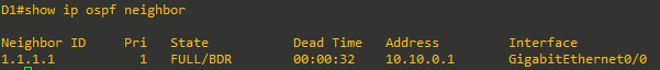
On D1, display the list of neighbors using the
show ip ospf neighborscommand.
The output confirms that R1 (i.e., 1.1.1.1) is a neighbor and is the BDR on the link. Therefore, D1 must be the DR.
-
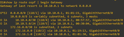
Verify the OSPF routing table using the
show ip router ospf | begin Gatewaycommand.
The routing table lists the four interarea networks and one external OSPF network.
-
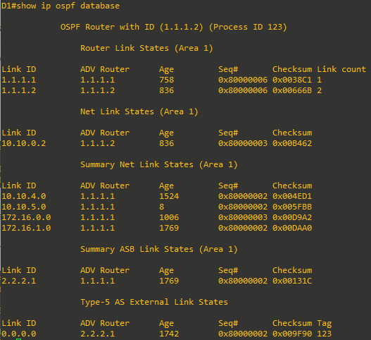
D1 learned about these networks from LSAs. A router maintains a LSDB for each area it has interfaces in. Because D1 is an internal OSPF router, it will only have entries for Area 1. To display the contents of the LSDB of D1, use the
show ip ospf databasecommand.
Notice how the command output is divided into the following five sections:
- Router Link States – These are the type 1 LSAs received by D1 and they identify the routers (i.e., 1.1.1.1 = R1, 1.1.1.2 = D1) in Area 1 that sent them, and the number of links that the routers have in the area. Therefore, R1 only has one interface in Area 1 and D1 has 2 interfaces in Area 1.
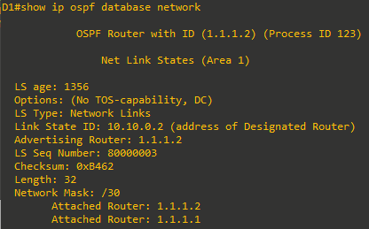
- Net Link States – These are the type 2 LSAs generated by the DR. In our example, the DR is 1.1.1.2 (i.e., D1) on the link 10.10.0.2.
- Summary Net Link States – These are the type 3 LSAs describing remote networks (i.e., our O IA networks or interarea routes) and the router that advertised them to D1.
- Summary ASB Link States – This is a type 4 LSA sent by the ABR (i.e., 1.1.1.1 = R1) advertising that there is an ASBR in the network (i.e., 2.2.2.1).
- Type-5 AS External Link States – This is a type 5 LSA advertising a default route (i.e., 0.0.0.0) and the router that is advertising it (i.e., 2.2.2.1).
-
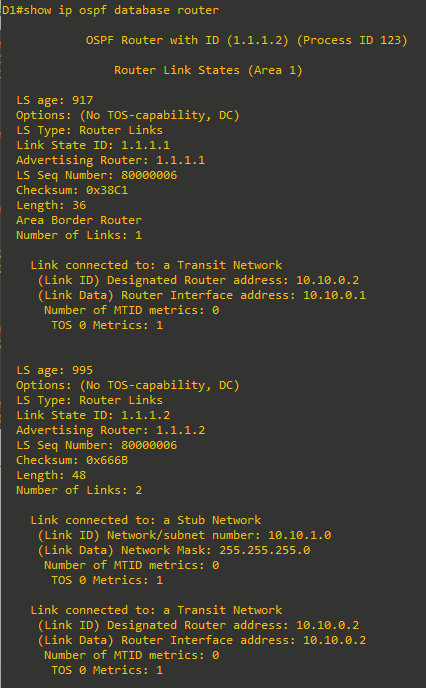
Additional information about the Router Link States type 1 LSA can be gathered using the
show ip ospf database routercommand.
The output provides more information about the type 1 LSAs. The first router link (i.e., type 1) LSA is from R1 (i.e., 1.1.1.1). It is an ABR with only 1 link in Area 1 which is the transit network connecting to D1. The second router link portion identifies the transit network connecting to R1 and the stub network of D1 (i.e., 10.10.1.0/24).
An OSPF link can be connected to a stub, to another router (point-to-point), or to a transit network. The transit network usually describes an Ethernet segment which can include two or more routers. If the link is connected to a transit network, the LSA also includes the IP address of the DR.
-
To learn more about type 2 network LSAs, use
show ip ospf database networkcommand.
The content of the type 2 LSA describes the network segment listing the DR address, the attached routers, and subnet mask using CIDR notation. This information is used by each router in the area to build the exact picture of the described multiaccess segment, which cannot be fully described with just type 1 LSAs.
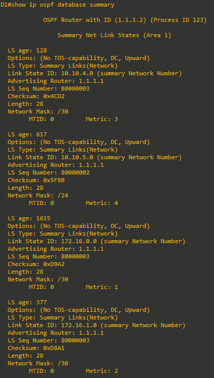
- To learn more about type 3 summary LSAs, use
show ip ospf database summarycommand.

The output lists four type 3 LSAs. The LSAs identify the interarea networks, which ABR advertised, and the network mask using CIDR notation.
-
To learn more about type 4 summary LSAs, use
show ip ospf database asbr-summarycommand.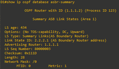
The output lists one type 4 LSA advertised by R1 identifying 2.2.2.1 as an ASBR.
-
Finally, to learn more about type 5 AS external link LSAs, use
show ip ospf database externalcommand.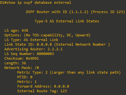
The output lists one type 5 LSA identifying that 0.0.0.0/0 is available from 2.2.2.1 (i.e., R2).


Step 2: Verifying OSPF and exploring LSAs on an ABR R1.
R1 is an ABR with interfaces in Area 1 and Area 0. Therefore, R1 will have two LSDBs.
Display the LSDB on R1.
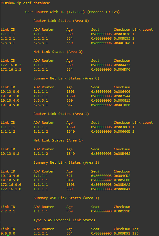
The output displays the type 1, 2, and 3 LSAs in Area 0, and then lists the type 1, 2, 3, and 4 LSAs in Area 1. The last section displays the type 5 LSAs.
To learn more about each LSA type, use the following commands:
show ip ospf database router
R1#show ip ospf database router

            OSPF Router with ID (1.1.1.1) (Process ID 123)

                Router Link States (Area 0)

  LS age: 1243
  Options: (No TOS-capability, DC)
  LS Type: Router Links
  Link State ID: 1.1.1.1
  Advertising Router: 1.1.1.1
  LS Seq Number: 80000005
  Checksum: 0x3078
  Length: 36
  Area Border Router
  Number of Links: 1

    Link connected to: a Transit Network
     (Link ID) Designated Router address: 172.16.0.2
     (Link Data) Router Interface address: 172.16.0.2
      Number of MTID metrics: 0
       TOS 0 Metrics: 1


  LS age: 1208
  Options: (No TOS-capability, DC)
  LS Type: Router Links
  Link State ID: 2.2.2.1
  Advertising Router: 2.2.2.1
  LS Seq Number: 80000008
  Checksum: 0xBE53
  Length: 48
  AS Boundary Router
  Number of Links: 2

    Link connected to: a Transit Network
     (Link ID) Designated Router address: 172.16.1.1
     (Link Data) Router Interface address: 172.16.1.1
      Number of MTID metrics: 0
       TOS 0 Metrics: 1

    Link connected to: a Transit Network
     (Link ID) Designated Router address: 172.16.0.2
     (Link Data) Router Interface address: 172.16.0.1
      Number of MTID metrics: 0
       TOS 0 Metrics: 1


  LS age: 1003
  Options: (No TOS-capability, DC)
  LS Type: Router Links
  Link State ID: 3.3.3.1
  Advertising Router: 3.3.3.1
  LS Seq Number: 80000006
  Checksum: 0xC1D8
  Length: 36
  Area Border Router
  Number of Links: 1

    Link connected to: a Transit Network
     (Link ID) Designated Router address: 172.16.1.1
     (Link Data) Router Interface address: 172.16.1.2
      Number of MTID metrics: 0
       TOS 0 Metrics: 1


                Router Link States (Area 1)

  LS age: 245
  Options: (No TOS-capability, DC)
  LS Type: Router Links
  Link State ID: 1.1.1.1
  Advertising Router: 1.1.1.1
  LS Seq Number: 80000007
  Checksum: 0x36C2
  Length: 36
  Area Border Router
  Number of Links: 1

    Link connected to: a Transit Network
     (Link ID) Designated Router address: 10.10.0.2
     (Link Data) Router Interface address: 10.10.0.1
      Number of MTID metrics: 0
       TOS 0 Metrics: 1


  LS age: 320
  Options: (No TOS-capability, DC)
  LS Type: Router Links
  Link State ID: 1.1.1.2
  Advertising Router: 1.1.1.2
  LS Seq Number: 80000007
  Checksum: 0x646C
  Length: 48
  Number of Links: 2

    Link connected to: a Stub Network
     (Link ID) Network/subnet number: 10.10.1.0
     (Link Data) Network Mask: 255.255.255.0
      Number of MTID metrics: 0
       TOS 0 Metrics: 1

    Link connected to: a Transit Network
     (Link ID) Designated Router address: 10.10.0.2
     (Link Data) Router Interface address: 10.10.0.2
      Number of MTID metrics: 0
       TOS 0 Metrics: 1


R1#
show ip ospf database network
R1#show ip ospf database network

            OSPF Router with ID (1.1.1.1) (Process ID 123)

                Net Link States (Area 0)

  LS age: 1264
  Options: (No TOS-capability, DC)
  LS Type: Network Links
  Link State ID: 172.16.0.2 (address of Designated Router)
  Advertising Router: 1.1.1.1
  LS Seq Number: 80000003
  Checksum: 0x4A23
  Length: 32
  Network Mask: /30
        Attached Router: 1.1.1.1
        Attached Router: 2.2.2.1

  LS age: 1229
  Options: (No TOS-capability, DC)
  LS Type: Network Links
  Link State ID: 172.16.1.1 (address of Designated Router)
  Advertising Router: 2.2.2.1
  LS Seq Number: 80000003
  Checksum: 0x6DF6
  Length: 32
  Network Mask: /30
        Attached Router: 2.2.2.1
        Attached Router: 3.3.3.1


                Net Link States (Area 1)

  LS age: 341
  Options: (No TOS-capability, DC)
  LS Type: Network Links
  Link State ID: 10.10.0.2 (address of Designated Router)
  Advertising Router: 1.1.1.2
  LS Seq Number: 80000004
  Checksum: 0xB263
  Length: 32
  Network Mask: /30
        Attached Router: 1.1.1.2
        Attached Router: 1.1.1.1
show ip ospf database summary
R1#show ip ospf database summary

            OSPF Router with ID (1.1.1.1) (Process ID 123)

                Summary Net Link States (Area 0)

  LS age: 562
  Options: (No TOS-capability, DC, Upward)
  LS Type: Summary Links(Network)
  Link State ID: 10.10.0.0 (summary Network Number)
  Advertising Router: 1.1.1.1
  LS Seq Number: 80000004
  Checksum: 0x62C1
  Length: 28
  Network Mask: /30
        MTID: 0         Metric: 1

  LS age: 303
  Options: (No TOS-capability, DC, Upward)
  LS Type: Summary Links(Network)
  Link State ID: 10.10.1.0 (summary Network Number)
  Advertising Router: 1.1.1.1
  LS Seq Number: 80000004
  Checksum: 0x73AB
  Length: 28
  Network Mask: /24
        MTID: 0         Metric: 2

  LS age: 1060
  Options: (No TOS-capability, DC, Upward)
  LS Type: Summary Links(Network)
  Link State ID: 10.10.4.0 (summary Network Number)
  Advertising Router: 3.3.3.1
  LS Seq Number: 80000003
  Checksum: 0x813
  Length: 28
  Network Mask: /30
        MTID: 0         Metric: 1

  LS age: 1578
  Options: (No TOS-capability, DC, Upward)
  LS Type: Summary Links(Network)
  Link State ID: 10.10.5.0 (summary Network Number)
  Advertising Router: 3.3.3.1
  LS Seq Number: 80000002
  Checksum: 0x1BFB
  Length: 28
  Network Mask: /24
        MTID: 0         Metric: 2


                Summary Net Link States (Area 1)

  LS age: 1051
  Options: (No TOS-capability, DC, Upward)
  LS Type: Summary Links(Network)
  Link State ID: 10.10.4.0 (summary Network Number)
  Advertising Router: 1.1.1.1
  LS Seq Number: 80000003
  Checksum: 0x4CD2
  Length: 28
  Network Mask: /30
        MTID: 0         Metric: 3

  LS age: 1541
  Options: (No TOS-capability, DC, Upward)
  LS Type: Summary Links(Network)
  Link State ID: 10.10.5.0 (summary Network Number)
  Advertising Router: 1.1.1.1
  LS Seq Number: 80000002
  Checksum: 0x5FBB
  Length: 28
  Network Mask: /24
        MTID: 0         Metric: 4

  LS age: 562
  Options: (No TOS-capability, DC, Upward)
  LS Type: Summary Links(Network)
  Link State ID: 172.16.0.0 (summary Network Number)
  Advertising Router: 1.1.1.1
  LS Seq Number: 80000004
  Checksum: 0xD7A3
  Length: 28
  Network Mask: /30
        MTID: 0         Metric: 1

  LS age: 1300
  Options: (No TOS-capability, DC, Upward)
  LS Type: Summary Links(Network)
  Link State ID: 172.16.1.0 (summary Network Number)
  Advertising Router: 1.1.1.1
  LS Seq Number: 80000003
  Checksum: 0xD8A1
  Length: 28
  Network Mask: /30
        MTID: 0         Metric: 2

R1#
show ip ospf database asbr-summary
R1#show ip ospf database asbr-summary

            OSPF Router with ID (1.1.1.1) (Process ID 123)

                Summary ASB Link States (Area 1)

  LS age: 1322
  Options: (No TOS-capability, DC, Upward)
  LS Type: Summary Links(AS Boundary Router)
  Link State ID: 2.2.2.1 (AS Boundary Router address)
  Advertising Router: 1.1.1.1
  LS Seq Number: 80000003
  Checksum: 0x111D
  Length: 28
  Network Mask: /0
        MTID: 0         Metric: 1
show ip ospf database external
R1# show ip ospf database external

            OSPF Router with ID (1.1.1.1) (Process ID 123)

                Type-5 AS External Link States

  LS age: 1309
  Options: (No TOS-capability, DC, Upward)
  LS Type: AS External Link
  Link State ID: 0.0.0.0 (External Network Number )
  Advertising Router: 2.2.2.1
  LS Seq Number: 80000003
  Checksum: 0x9D91
  Length: 36
  Network Mask: /0
        Metric Type: 2 (Larger than any link state path)
        MTID: 0
        Metric: 1
        Forward Address: 0.0.0.0
        External Route Tag: 123
Step 3: Verifying OSPF and exploring LSAs on the ASBR R2.
R2 is an ASBR with interfaces in Area 0 and an external non-OSPF network.
Display the LSDB on R2.
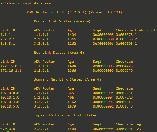
The output displays the type 1, 2, 3 and 5 LSAs in Area 0. Notice that there is no type 4 LSA because R2 is the ASBR and only an ABR can generate an LSA4.